Nearest neighbors with NDPointIndex#
Tip
New to spatial trees? Start with Tree-Based Indexing to learn how tree structures enable fast nearest-neighbor search, and when you need alternatives like Ball trees for geographic data.
Highlights#
xarray.indexes.NDPointIndexis useful for dealing with n-dimensional coordinate variables representing irregular data.It enables efficient point-wise (nearest-neighbors) data selection using Xarray’s advanced indexing capabilities.
By default, a
scipy.spatial.KDTreeis used under the hood for fast lookup of point data. Although experimental, it is possible to plug in alternative structures toNDPointIndex(See Advanced usage).
Basic usage#
A common task: you have scattered observations and want to color a regular grid based on the nearest observation at each grid point. This requires finding the nearest neighbor for every grid cell.
Let’s create some scattered measurements:
shape = (5, 10)
xx = xr.DataArray(
    np.random.uniform(0, 10, size=shape), dims=("y", "x")
)
yy = xr.DataArray(
    np.random.uniform(0, 5, size=shape), dims=("y", "x")
)
data = (xx - 5) ** 2 + (yy - 2.5) ** 2

ds = xr.Dataset(data_vars={"data": data}, coords={"xx": xx, "yy": yy})
ds
<xarray.Dataset> Size: 1kB
Dimensions:  (y: 5, x: 10)
Coordinates:
    xx       (y, x) float64 400B 1.636 5.304 8.267 8.642 ... 4.706 2.265 9.191
    yy       (y, x) float64 400B 3.925 4.306 2.534 4.908 ... 2.678 4.991 2.931
Dimensions without coordinates: y, x
Data variables:
    data     (y, x) float64 400B 13.35 3.356 10.67 19.06 ... 0.1181 13.69 17.75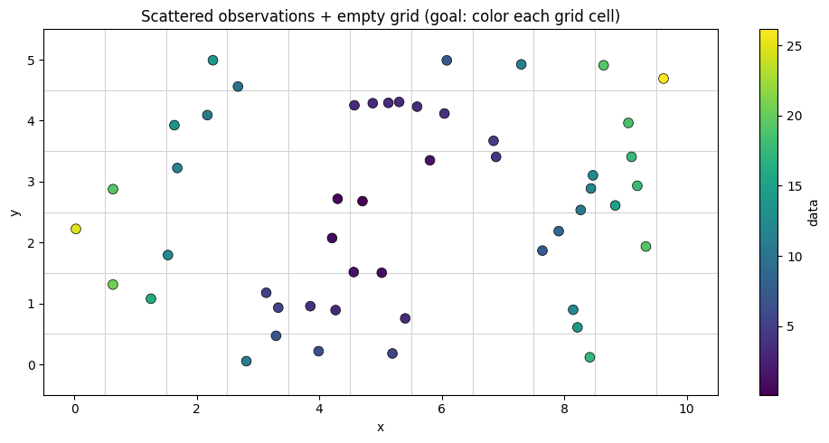
Assigning the index#
To enable nearest-neighbor lookups, we attach an NDPointIndex to our coordinate variables using set_xindex. This builds a KD-tree from the coordinate values, which will be used for efficient spatial queries.
The tuple ("xx", "yy") tells xarray which coordinates to combine into a multi-dimensional index.
Note
The tree is built once when you call set_xindex. This has a small upfront cost, but all subsequent queries are fast. This makes NDPointIndex ideal when you need to query the same dataset many times.
ds_index = ds.set_xindex(("xx", "yy"), xr.indexes.NDPointIndex)
ds_index
<xarray.Dataset> Size: 1kB
Dimensions:  (y: 5, x: 10)
Coordinates:
  * xx       (y, x) float64 400B 1.636 5.304 8.267 8.642 ... 4.706 2.265 9.191
  * yy       (y, x) float64 400B 3.925 4.306 2.534 4.908 ... 2.678 4.991 2.931
Dimensions without coordinates: y, x
Data variables:
    data     (y, x) float64 400B 13.35 3.356 10.67 19.06 ... 0.1181 13.69 17.75
Indexes:
  ┌ xx       NDPointIndex (ScipyKDTreeAdapter)
└ yyQuerying the index#
Now we can query for nearest neighbors using familiar xarray syntax. Under the hood, .sel(..., method="nearest") calls KDTree.query to efficiently find the closest point:
ds_index.sel(xx=3.4, yy=4.2, method="nearest")
<xarray.Dataset> Size: 24B
Dimensions:  ()
Coordinates:
    xx       float64 8B 2.674
    yy       float64 8B 4.56
Data variables:
    data     float64 8B 9.654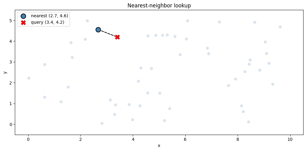
Assigning values from scattered points to a grid#
Sometimes you need to transfer scattered observations onto a regular grid. The simplest approach is nearest-neighbor lookup: each grid cell gets the value of its closest observation.
Note
This is not interpolation—there’s no averaging or blending. Each grid cell simply takes the value of one source point.
Without a spatial index, finding nearest neighbors requires n_grid × n_points comparisons (2,500 for 50 grid cells and 50 points). With NDPointIndex, each lookup is O(log n).
Let’s assign values to a 10×5 grid from our 50 scattered observations:
# create a regular grid as query points
ds_grid = xr.Dataset(coords={"x": range(10), "y": range(5)})

# selection supports broadcasting of the input labels
ds_selection = ds_index.sel(
    xx=ds_grid.x, yy=ds_grid.y, method="nearest"
)

# assign selection results to the grid
# -> nearest neighbor interpolation
ds_grid["data"] = ds_selection.data.variable

ds_grid
<xarray.Dataset> Size: 520B
Dimensions:  (x: 10, y: 5)
Coordinates:
  * x        (x) int64 80B 0 1 2 3 4 5 6 7 8 9
  * y        (y) int64 40B 0 1 2 3 4
Data variables:
    data     (x, y) float64 400B 20.49 20.49 24.79 19.21 ... 19.09 17.75 18.51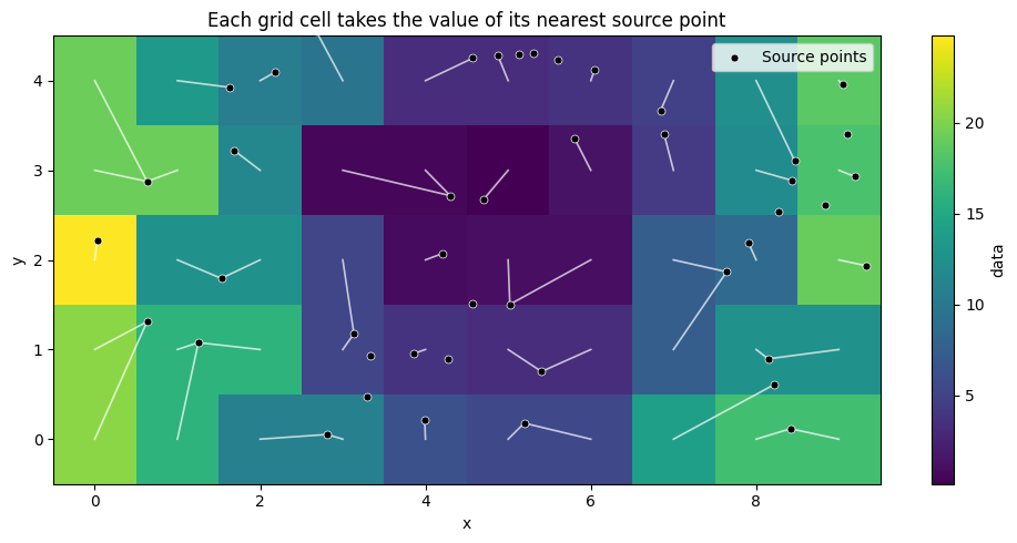
Advanced usage#
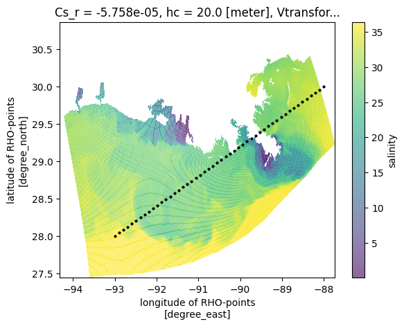
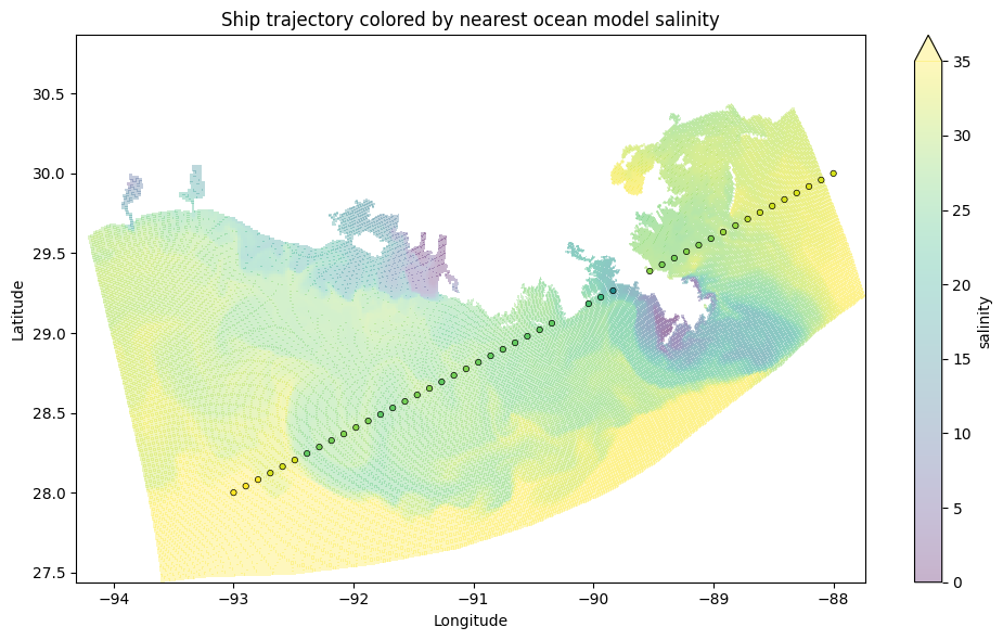
A real-world use case: you have ocean model output on a curvilinear grid and want to color a trajectory based on the nearest model values.
This example uses the Regional Ocean Modeling System (ROMS) Xarray example. The data is on a grid of eta_rho × xi_rho (20 × 40 = 800 points), but we want to query by lat_rho and lon_rho.
ds_roms = xr.tutorial.open_dataset("ROMS_example")
ds_roms
<xarray.Dataset> Size: 19MB
Dimensions:     (ocean_time: 2, s_rho: 30, eta_rho: 191, xi_rho: 371)
Coordinates:
  * ocean_time  (ocean_time) datetime64[ns] 16B 2001-08-01 2001-08-08
  * s_rho       (s_rho) float64 240B -0.9833 -0.95 -0.9167 ... -0.05 -0.01667
    Cs_r        (s_rho) float64 240B ...
    lon_rho     (eta_rho, xi_rho) float64 567kB ...
    h           (eta_rho, xi_rho) float64 567kB ...
    lat_rho     (eta_rho, xi_rho) float64 567kB ...
    hc          float64 8B ...
    Vtransform  int32 4B ...
Dimensions without coordinates: eta_rho, xi_rho
Data variables:
    salt        (ocean_time, s_rho, eta_rho, xi_rho) float32 17MB ...
    zeta        (ocean_time, eta_rho, xi_rho) float32 567kB ...
Attributes: (12/34)
    file:              ../output_20yr_obc/2001/ocean_his_0015.nc
    format:            netCDF-4/HDF5 file
    Conventions:       CF-1.4
    type:              ROMS/TOMS history file
    title:             TXLA ROMS hindcast run with dyes and oxygen
    rst_file:          ../output_20yr_obc/2001/ocean_rst.nc
    ...                ...
    compiler_flags:    -heap-arrays -fp-model fast -mt_mpi -ip -O3 -msse2 -free
    tiling:            010x012
    history:           Tue Jul 24 11:04:43 2018: /opt/nco/ncks -D 4 -t 8 /cop...
    ana_file:          /home/d.kobashi/TXLA_ROMS_reana/Functionals/ana_btflux...
    CPP_options:       TXLA2, ANA_BPFLUX, ANA_BSFLUX, ANA_BTFLUX, ANA_NUDGCOE...
NCO: netCDF Operators version 4.7.6-alpha04 (Homepage = htt...The challenge#
We want to color 50 trajectory points based on the nearest of 800 ocean model grid points.
Without a KD-tree: 50 × 800 = 40,000 distance calculations
With NDPointIndex: 50 × ~10 = ~500 calculations (80x faster!)
Assigning the Index#
First add the index to the lat and lon coord variable using set_xindex
ds_roms_index = ds_roms.set_xindex(
    ("lat_rho", "lon_rho"),
    xr.indexes.NDPointIndex,
)
ds_roms_index
<xarray.Dataset> Size: 19MB
Dimensions:     (ocean_time: 2, s_rho: 30, eta_rho: 191, xi_rho: 371)
Coordinates:
  * ocean_time  (ocean_time) datetime64[ns] 16B 2001-08-01 2001-08-08
  * s_rho       (s_rho) float64 240B -0.9833 -0.95 -0.9167 ... -0.05 -0.01667
    Cs_r        (s_rho) float64 240B ...
    h           (eta_rho, xi_rho) float64 567kB ...
  * lat_rho     (eta_rho, xi_rho) float64 567kB 27.45 27.45 ... 30.85 30.86
  * lon_rho     (eta_rho, xi_rho) float64 567kB -93.6 -93.58 ... -88.88 -88.87
    hc          float64 8B ...
    Vtransform  int32 4B ...
Dimensions without coordinates: eta_rho, xi_rho
Data variables:
    salt        (ocean_time, s_rho, eta_rho, xi_rho) float32 17MB ...
    zeta        (ocean_time, eta_rho, xi_rho) float32 567kB ...
Indexes:
  ┌ lat_rho  NDPointIndex (ScipyKDTreeAdapter)
  └ lon_rho
Attributes: (12/34)
    file:              ../output_20yr_obc/2001/ocean_his_0015.nc
    format:            netCDF-4/HDF5 file
    Conventions:       CF-1.4
    type:              ROMS/TOMS history file
    title:             TXLA ROMS hindcast run with dyes and oxygen
    rst_file:          ../output_20yr_obc/2001/ocean_rst.nc
    ...                ...
    compiler_flags:    -heap-arrays -fp-model fast -mt_mpi -ip -O3 -msse2 -free
    tiling:            010x012
    history:           Tue Jul 24 11:04:43 2018: /opt/nco/ncks -D 4 -t 8 /cop...
    ana_file:          /home/d.kobashi/TXLA_ROMS_reana/Functionals/ana_btflux...
    CPP_options:       TXLA2, ANA_BPFLUX, ANA_BSFLUX, ANA_BTFLUX, ANA_NUDGCOE...
NCO: netCDF Operators version 4.7.6-alpha04 (Homepage = htt...Coloring the trajectory#
Now we can efficiently find the nearest ocean model point for each trajectory point:
ds_roms_selection = ds_roms_index.sel(
    lat_rho=ds_trajectory.lat,
    lon_rho=ds_trajectory.lon,
    method="nearest",
)
ds_roms_selection
<xarray.Dataset> Size: 14kB
Dimensions:     (ocean_time: 2, s_rho: 30, trajectory: 50)
Coordinates:
  * ocean_time  (ocean_time) datetime64[ns] 16B 2001-08-01 2001-08-08
  * s_rho       (s_rho) float64 240B -0.9833 -0.95 -0.9167 ... -0.05 -0.01667
    Cs_r        (s_rho) float64 240B ...
    h           (trajectory) float64 400B ...
    lat_rho     (trajectory) float64 400B 28.01 28.03 28.07 ... 29.96 29.95
    lon_rho     (trajectory) float64 400B -93.0 -92.9 -92.8 ... -88.11 -88.09
    hc          float64 8B ...
    Vtransform  int32 4B ...
Dimensions without coordinates: trajectory
Data variables:
    salt        (ocean_time, s_rho, trajectory) float32 12kB ...
    zeta        (ocean_time, trajectory) float32 400B ...
Attributes: (12/34)
    file:              ../output_20yr_obc/2001/ocean_his_0015.nc
    format:            netCDF-4/HDF5 file
    Conventions:       CF-1.4
    type:              ROMS/TOMS history file
    title:             TXLA ROMS hindcast run with dyes and oxygen
    rst_file:          ../output_20yr_obc/2001/ocean_rst.nc
    ...                ...
    compiler_flags:    -heap-arrays -fp-model fast -mt_mpi -ip -O3 -msse2 -free
    tiling:            010x012
    history:           Tue Jul 24 11:04:43 2018: /opt/nco/ncks -D 4 -t 8 /cop...
    ana_file:          /home/d.kobashi/TXLA_ROMS_reana/Functionals/ana_btflux...
    CPP_options:       TXLA2, ANA_BPFLUX, ANA_BSFLUX, ANA_BTFLUX, ANA_NUDGCOE...
NCO: netCDF Operators version 4.7.6-alpha04 (Homepage = htt...The trajectory points are now colored by the salinity of the nearest ocean model grid point - efficiently computed using the KD-tree under the hood:
Alternative trees with xoak#
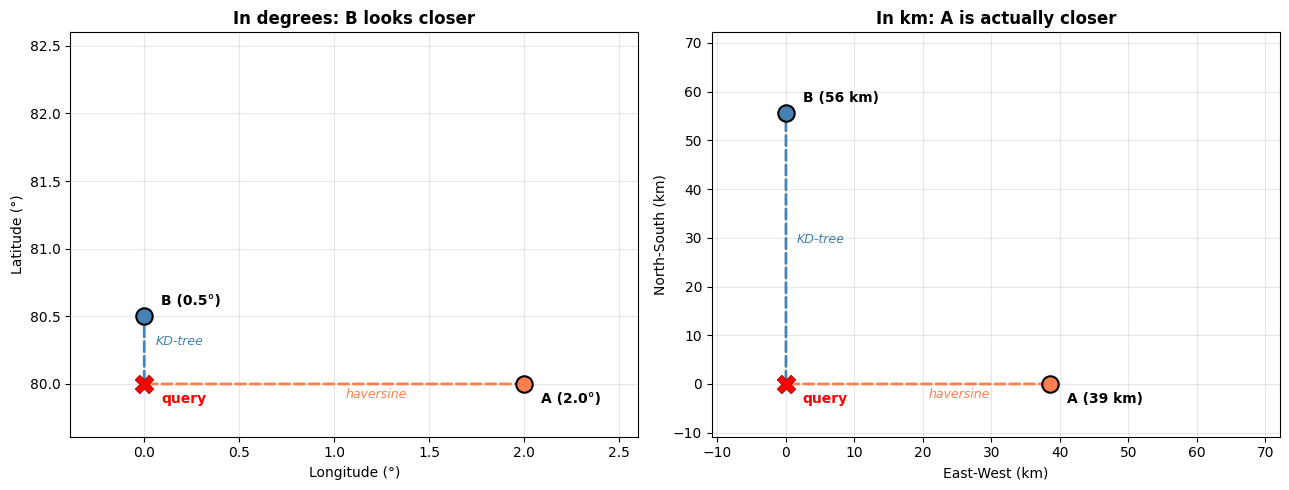
The default KD-tree uses Euclidean distance, which works well for most cases. However, for geographic coordinates (lat/lon), this can give incorrect results at high latitudes because longitude degrees shrink toward the poles.
Tip
See Tree-Based Indexing - The problem with geographic coordinates for a detailed explanation with visualizations.
Using a Ball tree for geographic data#
For accurate great-circle distance calculations, you can plug in a Ball tree with the haversine metric. The xoak package provides ready-made tree adapters for common use cases, including SklearnGeoBallTreeAdapter which wraps scikit-learn’s BallTree with the haversine metric.
Pass it as the tree_adapter_cls argument to set_xindex — everything else stays the same:
from xoak import SklearnGeoBallTreeAdapter

ds_roms_ball_index = ds_roms.set_xindex(
    ("lat_rho", "lon_rho"),
    xr.indexes.NDPointIndex,
    tree_adapter_cls=SklearnGeoBallTreeAdapter,
)
ds_roms_ball_index
<xarray.Dataset> Size: 19MB
Dimensions:     (ocean_time: 2, s_rho: 30, eta_rho: 191, xi_rho: 371)
Coordinates:
  * ocean_time  (ocean_time) datetime64[ns] 16B 2001-08-01 2001-08-08
  * s_rho       (s_rho) float64 240B -0.9833 -0.95 -0.9167 ... -0.05 -0.01667
    Cs_r        (s_rho) float64 240B ...
    h           (eta_rho, xi_rho) float64 567kB ...
  * lat_rho     (eta_rho, xi_rho) float64 567kB 27.45 27.45 ... 30.85 30.86
  * lon_rho     (eta_rho, xi_rho) float64 567kB -93.6 -93.58 ... -88.88 -88.87
    hc          float64 8B ...
    Vtransform  int32 4B ...
Dimensions without coordinates: eta_rho, xi_rho
Data variables:
    salt        (ocean_time, s_rho, eta_rho, xi_rho) float32 17MB ...
    zeta        (ocean_time, eta_rho, xi_rho) float32 567kB ...
Indexes:
  ┌ lat_rho  NDPointIndex (SklearnGeoBallTreeAdapter)
  └ lon_rho
Attributes: (12/34)
    file:              ../output_20yr_obc/2001/ocean_his_0015.nc
    format:            netCDF-4/HDF5 file
    Conventions:       CF-1.4
    type:              ROMS/TOMS history file
    title:             TXLA ROMS hindcast run with dyes and oxygen
    rst_file:          ../output_20yr_obc/2001/ocean_rst.nc
    ...                ...
    compiler_flags:    -heap-arrays -fp-model fast -mt_mpi -ip -O3 -msse2 -free
    tiling:            010x012
    history:           Tue Jul 24 11:04:43 2018: /opt/nco/ncks -D 4 -t 8 /cop...
    ana_file:          /home/d.kobashi/TXLA_ROMS_reana/Functionals/ana_btflux...
    CPP_options:       TXLA2, ANA_BPFLUX, ANA_BSFLUX, ANA_BTFLUX, ANA_NUDGCOE...
NCO: netCDF Operators version 4.7.6-alpha04 (Homepage = htt...The adapter handles converting lat/lon from degrees to radians internally, so you can query with the same degree-valued coordinates as before.
At high latitudes, longitude degrees are much shorter than latitude degrees. A KD-tree and Ball tree can pick different nearest neighbors for the same query:
Performance comparison#
Let’s compare the actual lookup times for our trajectory query:
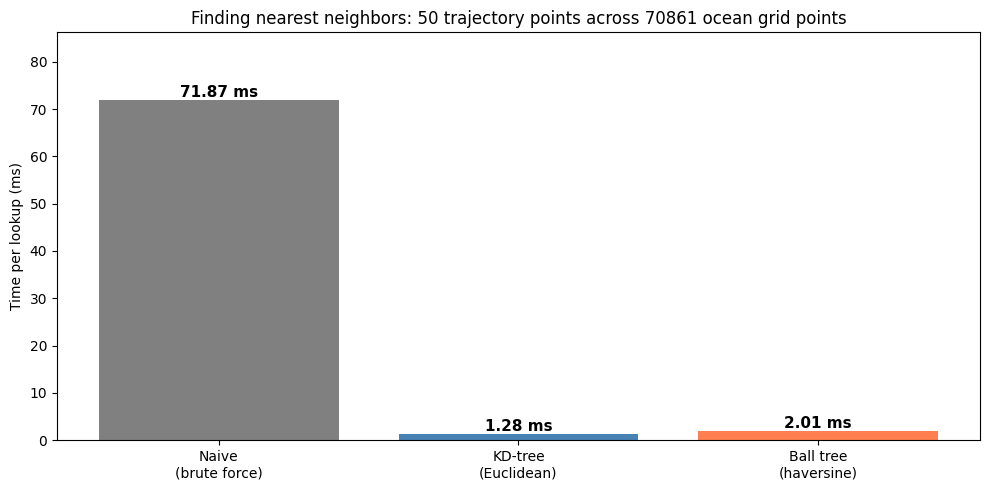
KD-tree is 55.9x faster than naive
Ball tree is 35.7x faster than naive

The tradeoff: KD-tree is faster but treats lat/lon as flat.
Ball tree is slower but uses haversine for correct great-circle distances.
Choosing a tree#
Use case |
Recommended |
Why |
|---|---|---|
Cartesian coordinates (x, y in meters) |
KD-tree (default) |
Fastest option, Euclidean distance is correct |
Geographic data near the equator |
KD-tree |
Euclidean on lat/lon is approximately correct |
Geographic data at high latitudes |
Ball tree with haversine |
Euclidean on lat/lon gives wrong answers |
Custom distance metric needed |
Ball tree |
Supports haversine, Manhattan, and others |
Very high dimensions (>20) |
Ball tree |
KD-trees degrade in high dimensions |
See also
Tree-Based Indexing for a visual explanation of how these tree structures work and why haversine matters for geographic data.
Building custom tree adapters for advanced use cases like implementing your own
TreeAdapter.