Raster affine transforms with rasterix.RasterIndex#

See also
Learn more at the Rasterix documentation page.
Highlights#
Rasterix provides a RasterIndex that allows indexing using a functional transformation defined by an affine transform.
It uses CoordinateTransformIndex as a building block (see Functional transformations with CoordinateTransformIndex). In doing so,
RasterIndex eliminates an entire class of bugs where Xarray allows you to add (for example) two datasets with different affine transforms (and/or projections) and return nonsensical outputs.
The associated coordinate variables are lazy, and use very little memory. Thus very large coordinate frames can be represented.
Rasterix uses a function rasterix.assign_index().
Example#
Here is a GeoTIFF file opened with rioxarray. GeoTIFF files do not contain explicit coordinate arrays, instead they commonly store the coefficients of an affine transform that software libraries use to calculate the coordinates.
On reading, we set "parse_coordinates": False to tell rioxarray to not generate coordinate variables.
import rasterix
import xarray as xr

xr.set_options(display_expand_indexes=True, display_expand_attrs=False, display_expand_data=False)

source = "https://noaadata.apps.nsidc.org/NOAA/G02135/south/daily/geotiff/2024/01_Jan/S_20240101_concentration_v4.0.tif"

da = xr.open_dataarray(source, engine="rasterio", backend_kwargs={"parse_coordinates": False})
da
<xarray.DataArray 'band_data' (band: 1, y: 332, x: 316)> Size: 420kB
[104912 values with dtype=float32]
Coordinates:
  * band         (band) int64 8B 1
    spatial_ref  int64 8B ...
Dimensions without coordinates: y, x
Attributes: (1)Notice how there are two dimensions x and y, but no coordinates associated with them.,
The affine transform information is stored in the attributes of spatial_ref under the name "GeoTransform"
da.spatial_ref.attrs
{'crs_wkt': 'PROJCS["NSIDC Sea Ice Polar Stereographic South",GEOGCS["Hughes 1980",DATUM["Hughes_1980",SPHEROID["Hughes 1980",6378273,298.279411123064,AUTHORITY["EPSG","7058"]],AUTHORITY["EPSG","1359"]],PRIMEM["Greenwich",0,AUTHORITY["EPSG","8901"]],UNIT["degree",0.0174532925199433,AUTHORITY["EPSG","9122"]],AUTHORITY["EPSG","10345"]],PROJECTION["Polar_Stereographic"],PARAMETER["latitude_of_origin",-70],PARAMETER["central_meridian",0],PARAMETER["false_easting",0],PARAMETER["false_northing",0],UNIT["metre",1,AUTHORITY["EPSG","9001"]],AXIS["Easting",NORTH],AXIS["Northing",NORTH],AUTHORITY["EPSG","3412"]]',
 'semi_major_axis': 6378273.0,
 'semi_minor_axis': 6356889.449,
 'inverse_flattening': 298.279411123064,
 'reference_ellipsoid_name': 'Hughes 1980',
 'longitude_of_prime_meridian': 0.0,
 'prime_meridian_name': 'Greenwich',
 'geographic_crs_name': 'Hughes 1980',
 'horizontal_datum_name': 'Hughes 1980',
 'projected_crs_name': 'NSIDC Sea Ice Polar Stereographic South',
 'grid_mapping_name': 'polar_stereographic',
 'standard_parallel': -70.0,
 'straight_vertical_longitude_from_pole': 0.0,
 'false_easting': 0.0,
 'false_northing': 0.0,
 'spatial_ref': 'PROJCS["NSIDC Sea Ice Polar Stereographic South",GEOGCS["Hughes 1980",DATUM["Hughes_1980",SPHEROID["Hughes 1980",6378273,298.279411123064,AUTHORITY["EPSG","7058"]],AUTHORITY["EPSG","1359"]],PRIMEM["Greenwich",0,AUTHORITY["EPSG","8901"]],UNIT["degree",0.0174532925199433,AUTHORITY["EPSG","9122"]],AUTHORITY["EPSG","10345"]],PROJECTION["Polar_Stereographic"],PARAMETER["latitude_of_origin",-70],PARAMETER["central_meridian",0],PARAMETER["false_easting",0],PARAMETER["false_northing",0],UNIT["metre",1,AUTHORITY["EPSG","9001"]],AXIS["Easting",NORTH],AXIS["Northing",NORTH],AUTHORITY["EPSG","3412"]]',
 'GeoTransform': '-3950000.0 25000.0 0.0 4350000.0 0.0 -25000.0'}
Assignment#
Rasterix provides a helpful assign_index function to automate the process of creating an index
da = rasterix.assign_index(da)
da
<xarray.DataArray 'band_data' (band: 1, y: 332, x: 316)> Size: 420kB
[104912 values with dtype=float32]
Coordinates:
  * band         (band) int64 8B 1
  * y            (y) float64 3kB 4.338e+06 4.312e+06 ... -3.912e+06 -3.938e+06
  * x            (x) float64 3kB -3.938e+06 -3.912e+06 ... 3.912e+06 3.938e+06
    spatial_ref  int64 8B ...
Indexes:
  ┌ x        RasterIndex (crs=None)
  └ y
Attributes: (1)We now have coordinate values, lazily generated on demand!
Indexing#
Slicing this dataset preserves the RasterIndex, though with a new transform
<xarray.DataArray 'band_data' (band: 1, y: 100, x: 100)> Size: 40kB
[10000 values with dtype=float32]
Coordinates:
  * band         (band) int64 8B 1
  * y            (y) float64 800B -6.625e+05 -6.875e+05 ... -3.138e+06
  * x            (x) float64 800B -1.438e+06 -1.412e+06 ... 1.012e+06 1.038e+06
    spatial_ref  int64 8B ...
Indexes:
  ┌ x        RasterIndex (crs=None)
  └ y
Attributes: (1)Compare the underlying transforms:
sliced.xindexes["x"].transform(), da.xindexes["x"].transform()
(Affine(25000.0, 0.0, -1450000.0,
        0.0, -25000.0, -650000.0),
 Affine(25000.0, 0.0, -3950000.0,
        0.0, -25000.0, 4350000.0))
Combining#
The affine transform is also used for alignment, and combining!
Here is a simple example. We slice the input dataset in to two
Let’s look at the bounding boxes for the sliced datasets
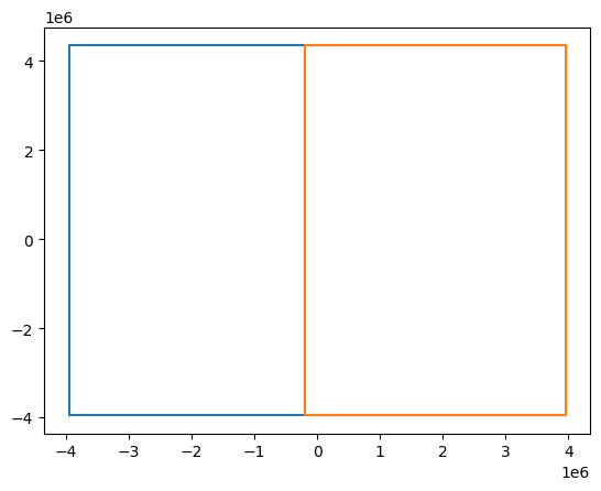
Concatenating these two along x preserves the RasterIndex!
combined = xr.concat([left, right], dim="x")
combined
<xarray.DataArray 'band_data' (band: 1, y: 332, x: 316)> Size: 420kB
0.0 0.0 0.0 0.0 0.0 0.0 0.0 0.0 0.0 0.0 ... 0.0 0.0 0.0 0.0 0.0 0.0 0.0 0.0 0.0
Coordinates:
  * band         (band) int64 8B 1
  * y            (y) float64 3kB 4.338e+06 4.312e+06 ... -3.912e+06 -3.938e+06
  * x            (x) float64 3kB -3.938e+06 -3.912e+06 ... 3.912e+06 3.938e+06
    spatial_ref  int64 8B 0
Indexes:
  ┌ x        RasterIndex (crs=None)
  └ y
Attributes: (1)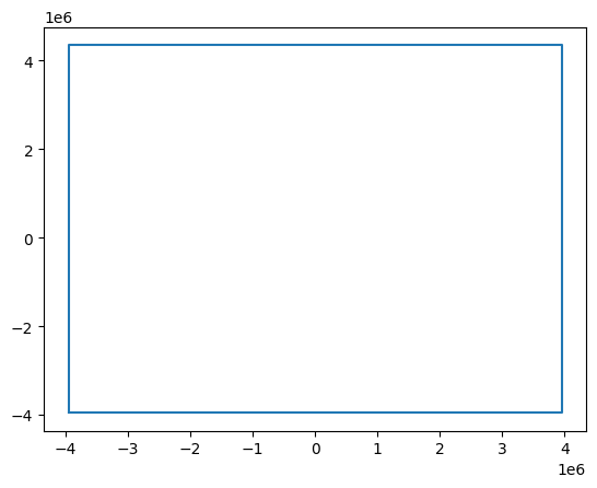
The coordinates on the combined dataset is equal to the original dataset
combined.xindexes["x"].equals(da.xindexes["x"])
True
This functionality extends to multi-dimensional tiling using xarray.combine_nested() too!
Tracking the affine transform#
Let’s reopen the same GeoTIFF file using rioxarray (without assigning a raster
index), slice both the x and y dimensions with steps > 1 and get the affine
transform parameters via rioxarray:
temp = xr.open_dataarray(source, engine="rasterio")
subset_a = temp.isel(x=slice(100, 200, 10), y=slice(200, 300, 20))
subset_a.rio.transform()
Affine(25000.0, 0.0, -1450000.0,
       0.0, -25000.0, -650000.0)
Rioxarray calculates the affine parameters of a dataarray by looking at the coordinate data and/or metadata. It maybe caches the results to avoid expensive computation, although in some cases like here a re-calculation seems to be needed:
subset_a.rio.transform(recalc=True)
Affine(250000.0, 0.0, -1562500.0,
       0.0, -500000.0, -412500.0)
The raster index added above eliminates the need to (re)calculate and/or cache the affine parameters from coordinate data after an operation on the dataaarray. Instead, it tracks and compute affine parameter values during the operation and generates (on-demand) coordinate data from these new parameter values: