Weather forecast cubes with rolodex.ForecastIndex#
See also
Learn more at the rolodex documentation.
One way to model forecast output is a datacube with four dimensions :
2 spatial dimensions
xandy,a forecast reference time (or initialization time) commonly
time[datetime64], anda forecast period or “timesteps in to the future” commonly
step[timedelta64]
There is one ancillary variable: ‘valid time’ which is the time for which the forecast is made: valid_time = time + step
Note
Note that not all forecast model runs are run for the same length of time! We could model these missing forecasts as NaN values in the output. A further complication is that different forecast systems have different output patterns, though most don’t have any missing output.
There are many ways one might index weather forecast output. These different ways of constructing views of a forecast data are called “Forecast Model Run Collections” (FMRC),
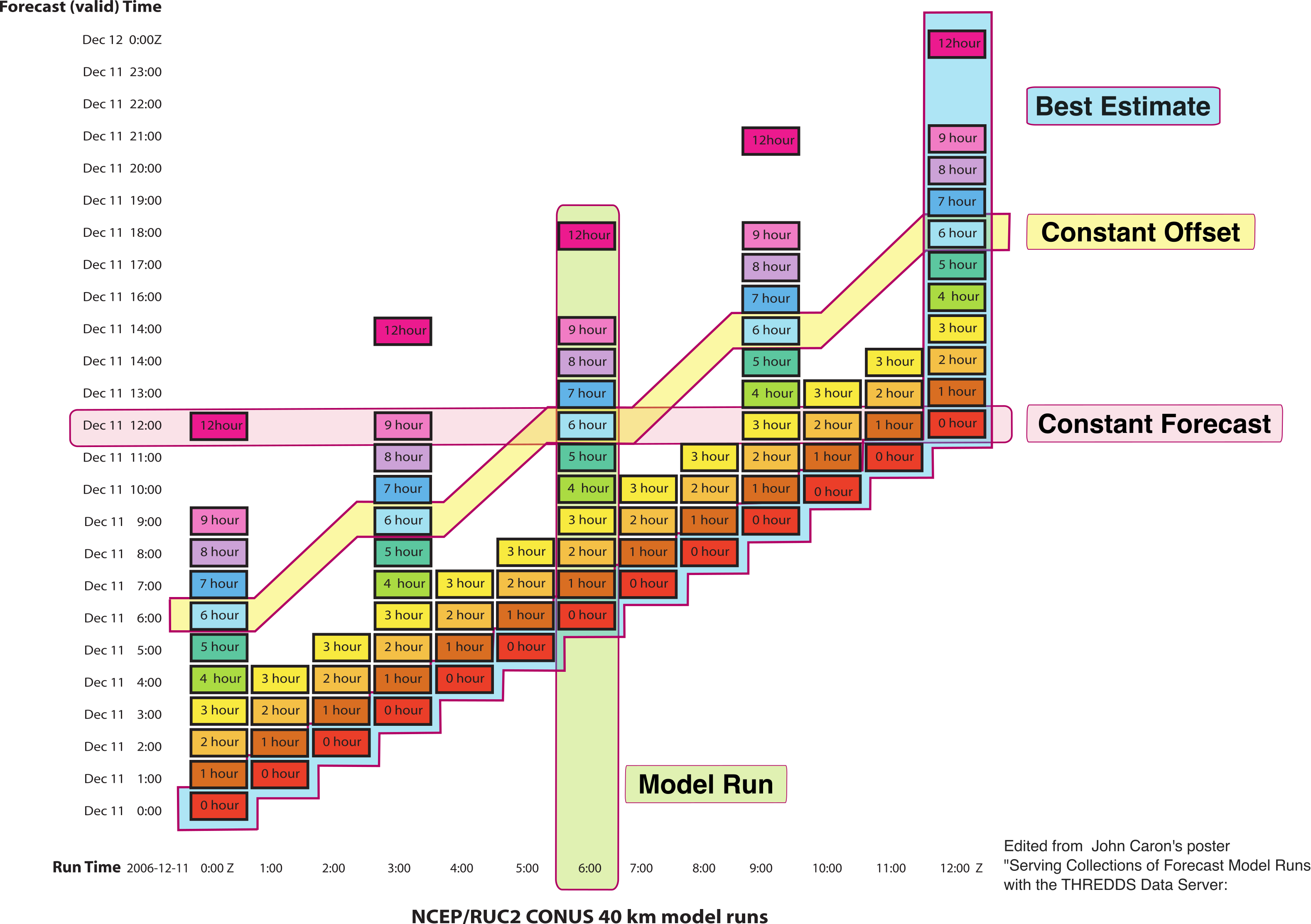
An illustration of different indexing patterns for weather forecast datasets. The y-axis is the ‘valid time’, and the x-axis is the ‘forecast reference or initialization time’. For a high-resolution schematic with expanded description of the different indexing patterns see the original PDF.#
“Model Run” : a single model run.
“Constant Offset” : all values for a given lead time.
“Constant Forecast” : all forecasts for a given time in the future.
“Best Estimate” : A best guess stitching together the analysis or initialization fields for past forecasts with the latest forecast.
Highlights#
All of these patterns are “vectorized indexing”, though generating the needed indexers is complicated by missing data.
ForecastIndex encapsulates this logic and,
Demonstrates how fairly complex indexing patterns can be abstracted away with a custom Index, and
Again illustrates the value of a custom Index in persisting “state” or extra metadata (here the type of model used “HRRR”).
Example#
Read an example dataset – downward short-wave radiation flux from the NOAA’s HRRR forecast system (High Resolution Rapid Refresh).
import rolodex.forecast
import xarray as xr

xr.set_options(display_expand_indexes=True, display_expand_data=False)

cube = xr.tutorial.open_dataset("hrrr-cube")
cube
/tmp/ipykernel_905/78795433.py:6: FutureWarning: In a future version, xarray will not decode the variable 'step' into a timedelta64 dtype based on the presence of a timedelta-like 'units' attribute by default. Instead it will rely on the presence of a timedelta64 'dtype' attribute, which is now xarray's default way of encoding timedelta64 values.
To continue decoding into a timedelta64 dtype, either set `decode_timedelta=True` when opening this dataset, or add the attribute `dtype='timedelta64[ns]'` to this variable on disk.
To opt-in to future behavior, set `decode_timedelta=False`.
  cube = xr.tutorial.open_dataset("hrrr-cube")
<xarray.Dataset> Size: 15MB
Dimensions:      (x: 80, y: 40, time: 24, step: 49)
Coordinates:
  * x            (x) float64 640B -8.975e+05 -8.945e+05 ... -6.605e+05
  * y            (y) float64 320B -2.731e+04 -2.431e+04 ... 8.669e+04 8.969e+04
  * time         (time) datetime64[ns] 192B 2025-01-01 ... 2025-01-01T23:00:00
  * step         (step) timedelta64[ns] 392B 00:00:00 ... 2 days 00:00:00
    spatial_ref  int64 8B ...
Data variables:
    dswrf        (x, y, time, step) float32 15MB ...
Attributes:
description: HRRR forecast datacube for one day, subset to a small box i...Assigning#
To assign we add a new variable: valid_time = time + step, “initialization time” + “time steps in to the future”.
from rolodex.forecast import Model, ForecastIndex

cube.coords["valid_time"] = rolodex.forecast.create_lazy_valid_time_variable(
    reference_time=cube.time, period=cube.step
)
With the valid_time array, we can illustrate the complex structure of this datacube.
green box illustrates the bounding box of valid forecast data, any white cells within this box are NaN — no forecast was generated for that forecast time with that initialization time.
the horizontal black line “2025-01-02 21:00” has 4 valid forecasts, though the underlying data has 23 data points (mostly NaN).
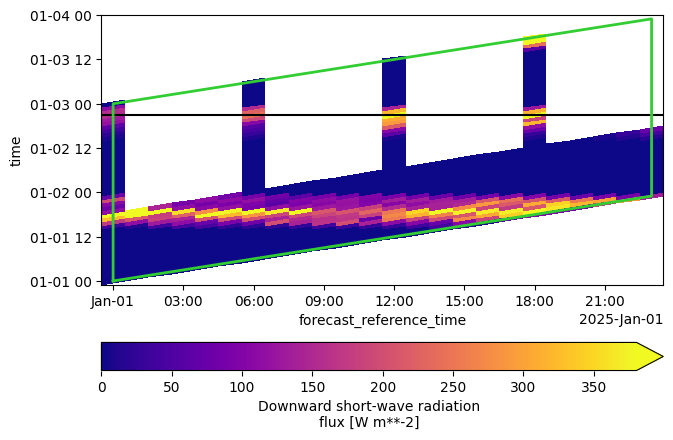
We will index out all forecasts for 2025-01-02 21:00, notice that there are 4 valid forecasts.
And then assign rolodex.ForecastIndex to time, step, valid_time.
We pass an optional custom kwarg model to indicate the type of forecast model used, here “HRRR”. ForecastIndex knows about HRRR’s output pattern.
cube = (
  cube.drop_indexes(["time", "step"])
  .set_xindex(
    ["time", "step", "valid_time"], ForecastIndex, model=Model.HRRR
  )
)
cube
<xarray.Dataset> Size: 15MB
Dimensions:      (x: 80, y: 40, time: 24, step: 49)
Coordinates:
  * x            (x) float64 640B -8.975e+05 -8.945e+05 ... -6.605e+05
  * y            (y) float64 320B -2.731e+04 -2.431e+04 ... 8.669e+04 8.969e+04
  * time         (time) datetime64[ns] 192B 2025-01-01 ... 2025-01-01T23:00:00
  * step         (step) timedelta64[ns] 392B 00:00:00 ... 2 days 00:00:00
  * valid_time   (time, step) datetime64[ns] 9kB ...
    spatial_ref  int64 8B ...
Data variables:
    dswrf        (x, y, time, step) float32 15MB ...
Indexes:
  ┌ time        ForecastIndex
  │ step
  └ valid_time
Attributes:
description: HRRR forecast datacube for one day, subset to a small box i...Indexing#
The usual indexing patterns along time and step individually still work.
<xarray.Dataset> Size: 3MB
Dimensions:      (x: 80, y: 40, time: 21, step: 11)
Coordinates:
  * x            (x) float64 640B -8.975e+05 -8.945e+05 ... -6.605e+05
  * y            (y) float64 320B -2.731e+04 -2.431e+04 ... 8.669e+04 8.969e+04
  * time         (time) datetime64[ns] 168B 2025-01-01T03:00:00 ... 2025-01-0...
  * step         (step) timedelta64[ns] 88B 02:00:00 03:00:00 ... 12:00:00
  * valid_time   (time, step) datetime64[ns] 2kB ...
    spatial_ref  int64 8B ...
Data variables:
    dswrf        (x, y, time, step) float32 3MB ...
Indexes:
  ┌ valid_time  ForecastIndex
  │ time
  └ step
Attributes:
description: HRRR forecast datacube for one day, subset to a small box i...FMRC Indexing#
rolodex provides dataclasses to indicate the type of indexing requested. We illustrate one of these: ConstantForecast which means
‘grab all forecasts available for this time.’
from rolodex.forecast import ConstantForecast
These can be used with sel to index along valid_time
subset = cube.sel(valid_time=ConstantForecast("2025-01-02T21:00"))
subset
<xarray.Dataset> Size: 52kB
Dimensions:      (x: 80, y: 40, time: 4)
Coordinates:
  * x            (x) float64 640B -8.975e+05 -8.945e+05 ... -6.605e+05
  * y            (y) float64 320B -2.731e+04 -2.431e+04 ... 8.669e+04 8.969e+04
  * time         (time) datetime64[ns] 32B 2025-01-01 ... 2025-01-01T18:00:00
    step         (time) timedelta64[ns] 32B 1 days 21:00:00 ... 1 days 03:00:00
    spatial_ref  int64 8B ...
    valid_time   datetime64[us] 8B 2025-01-02T21:00:00
Data variables:
    dswrf        (x, y, time) float32 51kB ...
Attributes:
description: HRRR forecast datacube for one day, subset to a small box i...On indeding, we receive 4 forecasts for this time (as expected)!
subset.dswrf.plot(col="time", cmap="plasma");
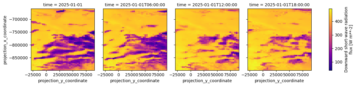
Note no NaNs or missing panels in the above output.